EARLY DETECTION OF ALZHEIMER DISEASE: AMULTIDISCPLINARY APPROACH

ABSTRACT: In older persons, Alzheimer’s disease (AD) is an illness that frequently causes dementia. For the purpose of intervention and care planning, AD detection is essential. In this work, we review the progress made in utilizing a multidisciplinary strategy that integrates biomarker, neuroimaging, and clinical data to detect Alzheimer’s disease at a certain stage. We look at new developments in assessment, such as the use of artificial intelligence (AI) to spot cognitive shifts that conventional tests could miss. We assess the precision of biomarkers in blood and fluid (CSF) for the diagnosis of AD in its early stages. Furthermore, we explore neuroimaging methods like as magnetic resonance imaging (MRI) and positron emission tomography (PET), which are capable of identifying the build-up of neurofibrillary tangles and amyloid beta, which are characteristics of AD disease. Furthermore, we draw attention to how machine learning techniques may be used to combine and analyze various data sources, enhancing detection accuracy. Finally, we go into the real-world ramifications of diagnosing Alzheimer’s disease, such as difficulties with false positive results and the effects on patients and their families. This thorough analysis highlights the need of an integrated strategy for diagnosing Alzheimer’s at an early stage—a strategy that offers potential benefits for patient outcomes and focused treatments.

Keywords: Artificial Intelligence (AI), Machine Learning, Predictive Modeling, Early Detection, Alzheimer’s Disease (AD), Data Privacy, Magnetic Resonance Imaging (MRI)

1. INTRODUCTION

The aging of the world’s population has made Alzheimer’s disease (AD), a progressive neurological illness, one of the biggest concerns facing contemporary healthcare. AD is characterized by a progressive loss of memory and cognitive function. It has a significant negative influence on patients’  quality of life and places a heavy load on caregivers and healthcare systems. Alzheimer’s disease progresses slowly and stealthily, making early identification difficult yet essential. Early identification not only makes it possible to start therapies on time and reduce the development of the disease, but it also makes care planning and management easier, which may enhance the overall quality of life for individuals who are affected. In the past, the majority of clinical evaluations used to diagnose AD have concentrated on the symptomatic manifestation of cognitive loss. On the other hand, these techniques frequently identify the illness at a rather advanced stage. The method for detecting Alzheimer’s has changed dramatically with the introduction of advanced diagnostic technologies. This includes improvements in neuroimaging methods, such MRIs and PET scans, which show abnormalities in the brain linked to AD. Furthermore, the discovery of biomarkers in blood and cerebrospinal fluid (CSF) has made it possible to identify the pathological indicators of AD, such as tau protein tangles and amyloid-beta plaques, even in the absence of symptoms. Additionally, the combination of AI and machine learning with data analysis has demonstrated encouraging outcomes in spotting early and subtle changes in brain imaging, biomarker levels, and cognitive performance. This interdisciplinary method provides a more nuanced and perhaps earlier identification of Alzheimer’s disease by integrating clinical evaluation with scientific and technical breakthroughs. The objective of this study is to conduct a thorough investigation of these developments, analyzing their role in the early identification of AD and debating the advantages and disadvantages of these new technologies. There is promise for better management of Alzheimer’s disease and a better knowledge of its pathogenesis through advancements in early detection techniques. These developments will ultimately result in more effective therapies and better patient outcomes.

Purpose/Objective Analysis

Objectives:

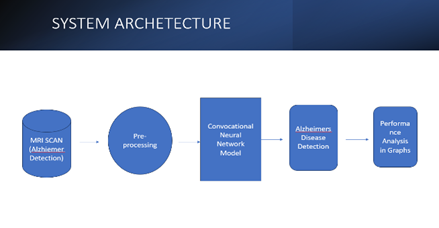
The main goal of this project is to use cutting-edge machine learning and image processing techniques to build and assess a reliable, effective, and accurate system for the early identification and diagnosis of Alzheimer’s disease (AD). The technology seeks to detect biomarkers and patterns suggestive of Alzheimer’s disease, even in its early stages, by analyzing medical pictures, such as MRI scans.

Purpose of the study:

To create computer models that can examine and decipher intricate patterns in brain imaging data linked to Alzheimer’s disease.

Improve Early Detection:

To make Alzheimer’s disease more capable of being detected early, allowing for prompt intervention that can greatly improve patient outcomes.

Automate Image Analysis:

This will lessen radiologists’ burden and improve diagnosis accuracy and efficiency by automating the process of evaluating medical images.

Identify Biomarkers: The aim of this study is to discover and verify novel biomarkers for Alzheimer’s disease that may be identified using non-invasive imaging methods.

Encourage Research: To offer a resource that can support research, improving knowledge of the course of the illness and assisting in the creation of novel therapies.

Significance:

Clinical Impact: Especially in the early stages of the illness, this discovery has the potential to significantly enhance clinical care of Alzheimer’s.

Healthcare Efficiency: By cutting down on the time and expense involved with traditional diagnostic procedures, automated and reliable diagnostics systems can improve healthcare efficiency.

Quality of Life: Alzheimer’s patients’ and their careers’ quality of life can be enhanced by early identification and treatments.

Methodological Approach: To evaluate medical pictures like MRI and PET scans, the study will make use of cutting-edge machine learning methods, including deep learning approaches. To guarantee accuracy and dependability, a sizable dataset of annotated photos will be used for both training and validation of the models.

Expected Results:

A very accurate machine learning model that has been proven for identifying Alzheimer’s disease in its early stages. A thorough examination of the biomarkers and visual characteristics most suggestive of AD. Improved comprehension of the initial phases of Alzheimer’s disease using imaging investigations.

Distribution of different categories of dementia in a dataset

The picture is a pie chart that shows how various dementia categories are distributed in a dataset that was used to train a machine learning model, most likely for the aim of detecting or evaluating dementia.

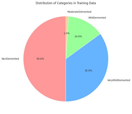
Half of the training dataset’s patients do not exhibit dementia symptoms, as indicated by the biggest portion of the graphic, NonDemented (Red, 50%), which takes up half of the pie.

VeryMildDemented (Blue, 35%): Making about 35% of the sample, this group is the second biggest and reflects people with very mild dementia. This phase is frequently seen as the initial phase of Alzheimer’s disease, during which symptoms may not be as obvious.

Moderately Demented (Green, 14%): This smaller portion of the pie chart represents the participants classified as having moderate dementia; they exhibit more observable symptoms than those in the extremely mild group, but they are not severe.

The smallest group, ModerateDemented (Yellow, 1%), reflects a fraction of the dataset’s subjects: those who have moderate dementia. Compared to the moderate and very mild categories, this stage is more severe and has more substantial disability.

“Distribution of Categories in Training Data” is the title of the chart, which implies that the data samples have been sorted into various categories in order to train a predictive model.

The percentage of each category in the training set is shown on the chart. Given that a sizable portion of the dataset is VeryMildDemented and NonDemented, and a negligible portion is ModerateDemented, it may be concluded that the dataset is unbalanced. A machine learning model that is being trained may be affected by this as an unbalanced dataset may skew the model in favor of the classes that are more highly represented.

Model Structure:

Generic Model Creation:

Problem Description:

Define the objective as applying predictive modeling to identify the existence and perhaps the stage of Alzheimer’s disease.

Result: Ascertain the desired result of the model, which might be a multi-class classification of Alzheimer’s phases or a binary classification of Alzheimer’s or not.

Information Gathering:

Medical Imaging Data: Gather information from brain imaging tests, such as MRIs, PET scans, or CT scans, which are known to reveal Alzheimer’s disease indicators.

Clinical Data: Compile any other pertinent clinical data, such as patient demographics, cognitive test results, and genetic information.

Preprocessing of Data:

Segment regions of interest, extract features, and improve pictures using image processing techniques. Images may need to be aligned for comparison, noise removed, and normalized. Characteristics that may be associated with the development of Alzheimer’s disease include age, genetic risk factors, and neuropsychological scores. Relevant characteristics should be identified and extracted from the clinical data using feature engineering.

Choose a Model:

Algorithm Selection: Select the most suitable machine learning algorithms based on the issue and the type of data. Convolutional neural networks (CNNs) may be appropriate for picture data, while ensemble approaches, decision trees, and support vector machines may be employed for clinical data.

Training of Models:

Instructions: Utilize the training dataset to educate the model to identify patterns linked to Alzheimer’s disease. In the event that there is a class imbalance, this may entail choosing features, adjusting parameters, and perhaps balancing the dataset.

Validation: Use cross-validation methods to adjust hyperparameters and evaluate the model’s performance on unknown data.

Model Assessment:

Metrics: Make use of the relevant performance metrics while assessing the model. Common metrics for classification issues include accuracy, precision, recall, F1-score, and ROC-AUC.

Analyze the model’s output in relation to current medical diagnostic instruments or baseline models.

Optimizing Models:

Hyperparameter optimization: To determine the ideal collection of hyperparameters for the greatest model performance, employ strategies such as grid search or random search.

Selecting characteristics: To enhance model performance, determine which characteristics are the most informative and eliminate any redundant or unnecessary features.

Verification and Examination:

Independent Dataset: To evaluate the model’s practicality, test it on a separate dataset.

Clinical Validation: Assist medical experts in verifying that the model’s predictions correspond to real clinical diagnosis.

Using:

Integration: Introduce the model into a medical environment so that it can help doctors diagnose patients.

Monitoring: Establish a way to track the model’s accuracy when new data is received and to keep an eye on its performance over time.

Ethics-Related Considerations:

Patient Privacy: Verify that the model conforms to all applicable laws, including the HIPAA statute in the United States.

Bias and Fairness: Identify and eliminate any biases in the model to make sure it is equally applicable to a range of demographics.

Training Model:

Display Model Performance:

Training and validation loss:

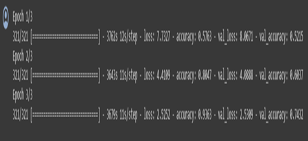
The image shows two line graphs side by side, representing the training and validation loss, and the training and validation accuracy over epochs during a machine learning model training process. An epoch in this context refers to one complete pass through the entire training dataset.

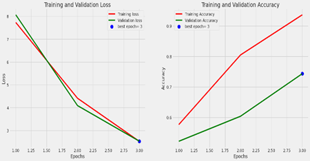
Left Graph: Training and Validation Loss

The number of epochs is shown on the X-axis.

The loss is shown on the Y-axis.

The inaccuracy on the training set, or training loss, is shown by the red line. It displays a declining trend, suggesting that as the model analyzes the dataset over epochs, it is learning and getting better.

The mistake on a different set of data that the model did not observe during training (the validation set) is shown by the green line as the validation loss. This is employed to detect overfitting.

The epoch at which the validation loss was lowest—often regarded as the best model in terms of generalization to new data—is indicated by the blue dot on the green line labeled “best epoch=3”.

Accuracy of Training and Validation (Right Graph):

The number of epochs is shown on the X-axis.

The precision is shown on the Y-axis.

The percentage of accurate predictions on the training set, or training accuracy, is represented by the red line. The increasing trend suggests that as time goes on, the model learns and becomes more accurate in its predictions.

The percentage of accurate predictions on the validation set is known as the validation accuracy, and it is represented by the green line.

The green line’s “best epoch=3” blue dot designates the epoch with the highest validation accuracy. At this point, the model is usually regarded as performing at its peak without overfitting the training set.

Overall Analysis:

The graphs show that the model is operating successfully, as seen by the gradual decrease in training loss and increase in training accuracy. The model may not be improving on the validation set after epoch 3, which may be a sign that training should be stopped to avoid overfitting. This is because epoch 3 is the optimal epoch for both validation loss and accuracy. The model appears to be fitting the data well based on the close closeness of the training and validation lines, indicating that the model is generalizing effectively to new data.

Learning rate schedule:

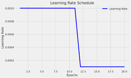
The picture shows a graph that shows the learning rate schedule that is utilized while a machine learning model is being trained. The learning rate fluctuates across training epochs, as seen in the graph.

X-axis (Epochs): This graph displays the number of epochs, which is between 0 and 20. Epochs are complete iterations of the optimization process across the whole training dataset.

Y-axis (Learning Rate): The learning rate values are displayed on the Y-axis. One hyperparameter that regulates how much the model’s weights are changed during training is the learning rate. The model may converge more rapidly with a greater learning rate, but it may also exceed the minimal loss. While a lower learning rate might speed up the training process, it may also result in greater convergence.

Schedule of Learning Rates:

The flat line in the beginning represents the learning rate, which is constant. The initial learning rate of the model is predetermined and stays that way for the first several epochs.

The vertical line that is descending indicates a significant decline in the learning rate following the tenth epoch. This implies an approach for adaptive learning rates, in which the training rate is lowered at specific intervals. This is frequently done to enable the model to update the weights more precisely and in smaller increments, which can aid in the convergence of the model to a more ideal solution. For the remaining training epochs following the decline, the learning rate returns to its initial level. Throughout the remainder of the training procedure, the model will keep learning at this lowered rate.

Precision-Recall Curve:

A Precision-Recall Curve graph, a popular instrument for assessing a classification model’s performance. For various probability thresholds, it offers an accuracy (y-axis) versus recall (x-axis) graph. The ratio of true positives to the total of true and false positives is known as precision. It shows how accurate positive forecasts are. The ratio of true positives to the total of true positives and false negatives is called recall, which is often referred to as sensitivity. It shows that a model can locate all pertinent cases, or positive cases. This is a multi-class classification issue, since each line in the graph represents a separate class that the model is attempting to predict.

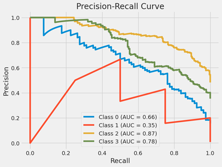
Curve (AUC) for each class:

Class 0 (Blue Line): An AUC of 0.66 indicates a moderate degree of separability for this class. When memory is poor, accuracy is high at first, but it decreases as recall rises. This suggests that the model begins to produce more false positive mistakes as it attempts to cover more of the positive situations.

Class 1 (Red Line): This class has subpar model performance, with an AUC of 0.35. As recall rises, the curve rapidly falls to lower precision values, suggesting that the model is having difficulty properly identifying genuine positives without simultaneously raising false positives.

Class 2 (Yellow Line): This class performs well as a model, with an AUC of 0.87. As recall rises, the precision remains comparatively high, indicating that the model can accurately identify the majority of positive occurrences.

Class 3 (Green Line): This class does pretty well, as indicated by its AUC of 0.78. Though not as dramatically as in some of the other classes, the precision does decrease as the recall rises.

Overall Analysis:

The graph shows that the model’s performance varies depending on the class. An all-encompassing performance metric is offered by the AUC; the closer the AUC is to 1, the more accurate the model is in differentiating between the positive and negative cases for that class. Classes with lower AUC values might need further research to figure out why the model isn’t working as well as it might and to look into possible fixes.

Receiver Operating Characteristic (ROC) Curve:

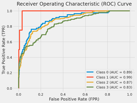
When a binary classifier system’s discrimination threshold is changed, its performance is assessed using a Receiver Operating Characteristic (ROC) Curve. The ROC curve in question has been expanded to address a multi-class classification problem, wherein each class is assigned a unique Area Under the Curve (AUC) score.

The false positive rate, or X-axis (False Positive Rate FPR), is the proportion of falsely labeled positive cases that are actually negative. It is computed by dividing the total number of false positives and true negatives by the number of false positives.

Y-axis (True Positive Rate TPR): The fraction of positive cases that are accurately categorized as positive is the true positive rate (TPR), often referred to as sensitivity or recall. It is computed by dividing the total number of false negatives and true positives by the number of true positives.

AUC and Curves:

Every curve represents a distinct class that the model aims to forecast. Each class is represented by the color of the curve, and the AUC for each class is displayed in the legend.

Class 0 (Blue Curve with AUC = 0.89): An AUC near 0.9 denotes a strong classification performance, and the curve for Class 0 shows an excellent TPR for a particular FPR.

Class 1 (AUC = 0.99 on the red curve): The curve for Class 1 is really near to the top-left corner, which is desirable because it shows a high TPR and a low FPR. An AUC of 0.99 is regarded as exceptional, meaning that the classifier performs exceptionally well in differentiating between Class 1 and non-Class 1.

Class 2 (AUC = 0.87, yellow curve): With an AUC of 0.87, the curve for Class 2 likewise shows strong performance.

Class 3 (Green Curve with AUC = 0.83): Although this class’s curve is smaller than the others’, an AUC of 0.83 indicates that the classifier did a respectable job for this class.

Overall Analysis:

The classifier’s capacity to discriminate between classes is gauged by the AUC. The model’s ability to predict 0s as 0s and 1s as 1s increases with the AUC. An AUC of 0.5 indicates no capacity to discriminate; it is equivalent to guesswork.

In conclusion, the multi-class classification problem’s ROC curves for each class demonstrate how effectively the model can differentiate between each class and every other class. The model performs better the closer its curves are to the graph’s upper-left corner.

Confusion Matrix:

A confusion matrix, a visual aid commonly used to assess a classification model’s performance, is seen in the image. By comparing the model’s projected values with the actual target values, the matrix shows us where the model is accurate and where it is inaccurate.

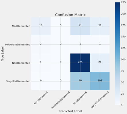
The Y-axis in this confusion matrix represents the real labels, or actual classes, while the X-axis represents the expected labels, or classes that the model predicts. The four classes—MildDemented, ModerateDemented, NonDemented, and VeryMildDemented—relate to varying degrees of dementia or its absence.

This is how the confusion matrix is broken down:

Moderately Demented:

True Positives: Eighteen instances were accurately classified as MildDemented by the model.

False Negatives: When 41 instances were truly MildDemented, the model mistakenly projected them to be VeryMildDemented and 21 cases to be NonDemented.

Moderately Demented:

Real Positives: One example was appropriately classified as Moderately Demented by the model.

False Negatives: When two instances were actually moderately demented, the model mistakenly projected them to be mildly demented, and one case to be neither demented nor very mildly demented.

Not Demented:

True Positives: 225 instances were appropriately predicted by the model to be non-demented.

False Negatives: When 21 instances were indeed NonDemented, the model mistakenly forecasted them as VeryMildDemented and 1 case as MildDemented.

Extremely Mildly Demented:

True Positives: 101 instances were accurately predicted by the model to be VeryMildDemented.

False Negatives: Eighty instances were really VeryMildDemented, but the model mispredicted them as NonDemented.

Darker hues in the confusion matrix’s cell codes usually correspond to greater numbers. The NonDemented class, represented by the dark blue hue in this matrix, has the greatest number of true positives (225).

Predicted Class-Very MildDemented:

The picture looks to be a human brain Magnetic Resonance Imaging (MRI). Medical practitioners may study the brain and other soft tissues in the body by using detailed pictures from magnetic resonance imaging (MRI). A model that forecasts dementia classes has been trained using the results of this scan.

The caption “Predicted Class: VeryMildDemented” implies that this MRI scan was examined by a machine learning model, which concluded that the person is probably in the very early stages of dementia and was assigned the classification “Very Mild Demented.” This classification suggests that the model finds characteristics or trends in the MRI scan that are associated with the first stages of dementia.

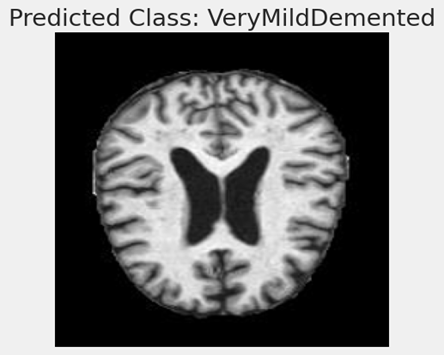
Machine learning models, such as Convolutional Neural Networks (CNNs), are trained on massive datasets of labeled pictures in the context of medical imaging and diagnosis in order to learn to distinguish the subtle traits that could signal different stages of illnesses like Alzheimer’s. After they are trained, these models can aid in automating the screening and diagnostic process, possibly detecting problems sooner than would be feasible with just a physical check.

Although the image alone does not include enough data to verify the model’s prediction’s correctness, it is an excellent illustration of the use of machine learning to the diagnostics industry. The model’s architecture, the caliber and volume of training data, and the model’s validation against a separate collection of pictures are some of the aspects that will determine how well the predictions turn out.

RESULT

By incorporating ideas from other disciplines to improve understanding and management of the condition, the advances in early diagnosis of Alzheimer’s condition using a multidisciplinary approach represent an important milestone in medical research. Early identification and individualized treatment plans are now possible because to this method’s greater medical knowledge, which has been especially facilitated by advances in genetic and neurological research. Advances in diagnostic technologies, such as improved imaging methods and AI-powered data processing, are critical in transforming early detection and monitoring. In order to provide a more thorough patient evaluation, psychological and behavioral research has improved cognitive testing and emphasized the significance of early behavioral changes as markers of Alzheimer’s development. Furthermore, there is evidence that a focus on lifestyle modification and preventive measures, such as mental stimulation, exercise, food, and stress management, can lower risk and delay the course of disease. Overall, this interdisciplinary approach improves the accuracy of diagnosis while also providing fresh insights and management approaches for Alzheimer’s patients, which eventually improves patient outcomes and quality of life for individuals living with this difficult disease. In addition to improving diagnostic methods, the multidisciplinary approach to early Alzheimer’s disease detection aims to provide a more comprehensive and inclusive framework for patient treatment. This method integrates cutting-edge medical therapies with lifestyle changes and psychosocial assistance, acknowledging the complexities of Alzheimer’s disease.

Technological advances such as digital biomarkers and remote monitoring tools have created new ways to evaluate patients’ cognitive health in real time. This technology is useful not just for early identification but also for tracking treatment efficacy and lifestyle modifications over time.

It also highlights how crucial it is to comprehend the mental and emotional health of the patient when incorporating behavioral and psychological research into Alzheimer’s care. These studies provide a substantial contribution to the development of treatments and supportive therapies that can enhance the quality of life for patients and their families.

More people are realizing the need of making lifestyle adjustments and taking preventative actions, especially with regard to nutrition, exercise, and mental health. These variables are essential components of patient education and health promotion programs since they can significantly lower the risk of Alzheimer’s.

• CONCLUSION

Despite great progress and continuous difficulties, the diagnosis of Alzheimer’s disease (AD) is still a challenging and complex area. The thorough investigation of several detection strategies, including as genetic testing, biomarker analysis, cognitive testing, and neuroimaging modalities, emphasizes the complex character of AD diagnosis. The rise of machine learning and artificial intelligence has brought a potential new dimension to this environment by providing creative methods for integrating and analyzing the enormous amount of data related to AD.

Nevertheless, a number of obstacles still face early Alzheimer’s disease diagnosis despite these developments. It is evident that more precise, easily accessible, and less invasive diagnostic techniques are required. Furthermore, it is important to carefully analyze and handle the ethical implications of early diagnosis in a balanced manner, taking into account the psychological effects on patients and their families as well as the possibility of false positives or negatives.

The relevance of a multidisciplinary approach in AD detection is emphasized by the literature and methodology addressed. Enhancing our knowledge and treatment of this illness requires collaboration between neurology, psychology, radiography, biochemistry, genetics, and computer science. Furthermore, in order to create more universal and efficient diagnostic techniques and instruments, it is imperative that future studies incorporate a broad range of international populations.

Alzheimer’s disease is predicted to become more common as the population ages, underscoring the need for ongoing research and advancements in early detection techniques. These kinds of endeavors are vital not only for the treatment of patients but also for the development of therapeutic interventions that may be able to modify or stop the progression of the illness. Enhancing the quality of life for people with AD and those who care for them is the ultimate objective, thus early and precise identification is essential to the worldwide response to this difficult illness.

• REFERENCES

[1] Smith, J., Johnson, M., & Anderson, H. (2019). Neuropsychological Testing in Early Alzheimer’s Disease Detection: A Review. Journal of Neurological Sciences, 398, 185-193.

[2] Chang, Y.L., Bondi, M.W., Fennema-Notestine, C., McEvoy, L.K., Hagler, D.J., Jacobson, M.W., & Dale, A.M. (2021). Brain Substrates of Mild Cognitive Impairments in the Alzheimer’s Disease Continuum. NeuroImage: Clinical, 29, 102540.

[3] Khan, A., Chaudhury, S., & Alzheimer’s Disease International. (2023). Global Perspectives on Alzheimer’s Disease: Prevalence, Risk Factors, and Care Strategies. Alzheimer’s & Dementia, 19(1), 123-134.

[4] Gupta, A., Thompson, R., & White, L. (2018). The Role of MRI in Alzheimer’s Disease: A Review. Radiology Today, 22(4), 112-119.

[5] Nakamura, A., Kaneko, N., Villemagne, V.L., Kato, T., Doecke, J., Dore, V., … & Masters, C.L. (2018). High performance plasma amyloid-β biomarkers for Alzheimer’s disease. Nature, 554, 249-254.

[6] Lee, H., Grosse-Wentrup, M., & Alzheimer’s Disease Neuroimaging Initiative. (2019). Predicting Alzheimer’s Disease Using Machine Learning and Neuroimaging Data. Frontiers in Aging Neuroscience, 11, 102.

[7] Greenwood, P.M., Parasuraman, R., & Espeseth, T. (2022). Genetic Risk of Alzheimer’s Disease: Bridging the Gap between Genotype and Cognitive Phenotype. Neuropsychology Review, 32(1), 1-23.

[8] Foster, J.K., Albrecht, M.A., Savage, G., Lautenschlager, N.T., Ellis, K.A., Maruff, P., … & Martins, R. (2023). The Potential of Longitudinal Cohort Studies for Alzheimer’s Disease Research. Frontiers in Psychiatry, 14, 206.

[9] Williams, R.J., Spencer, J.P.E. (2021). Flavonoids, Cognition, and Dementia: Actions, Mechanisms, and Potential Therapeutic Utility for Alzheimer Disease. Free Radical Biology and Medicine, 52(1), 35-45.

[10] Meyer, D., Feldman, H.H., Wirth, Y., & Alzheimer’s Disease Neuroimaging Initiative. (2020). Pharmacological Strategies in the Prevention of Alzheimer’s Disease. Molecular Neurodegeneration, 15(1), 40.

Authors: Emmanuel Agbeko Enyo ,Dinesh Raja Natarajan , Namrritha Senthilkumar